Lately, I have gotten interested in predictive maintenance and wonder how close are we in replacing preventive maintenance with predictive models. The more I read/thought about it the more I realized how much the answer hinges on the practice of keeping record of all piece replacements and maintenance, and engineering logs etc. and the whole thing became more and more overwhelming… Until I came across this -admittedly over simplified- set of -simulated- data and decided to start playing with it. The details of the simulations and some contextual information about the data are explained in a paper that I have only browsed very briefly and even now, have no idea what each of the columns I’ve worked with mean, but in a way this is part of the fun too.

About CMAPSS dataset

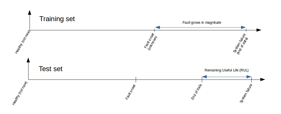
According to the README that comes with the dataset, the format of training and test sequences (for each engine with a separate id) looks like the schematics bellow. This also implies that we have more observations of systems that are critically close to their failure than those farther away from it. This could be our curse or blessing, depending on what we are interested in. If we are interested in spotting a failing system as soon as possible (but possibly with a larger margin of accuracy), this is not how we want our training and test set to look like. However, if we are interested in learning the exact behavior of the system after the first fault and the growth of the system failure, we could embrace this training set. Although the test set then may not be perfect for us. This will get clearer if we look at the actual distribution of RUL values (in cycle) for the training and test sets.

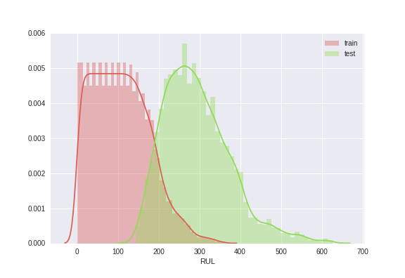
This relationship between labels of the training and test set looks a bit troublesome, how could we expect our model that is trained on the red plot, return reliable prediction of system on the green?

Regression or Classification

This brought me to the question of method, should I solve this as a regression problem, learn from the sequences my training data provides me with, and predict a value for the RUL together with the uncertainties, or should I try to learn/predict the health stage the engine is in, at each point in time? The former method is probably something to try on solving using a seq2seq method like an LSTM (or stacking a bunch of them), but for now I’m sticking to the classification approach.

Preprocessing

Like every other dataset, I started by just looking at my columns and their different statistical description/aggregation etc. to get an idea of what’s going on. This step is -obviously- quite experimental, but here is a bullet-point description of it that I found useful to document and look at every time I go back to o the same thing for new subsets of the data.

• Evaluate RULs from assumptions about the training set and label files for the test set
• Scale all features and labels
• Bin labels(RULs) into discrete classes
• Binary and one-hot encode labels (moved to the classification notebooks for clarity)
• PCA (since the EDA and a crude physical understanding of the system was telling me that most of these columns are probably very weakly related to what I’m interested in learning about the system - and I was right)

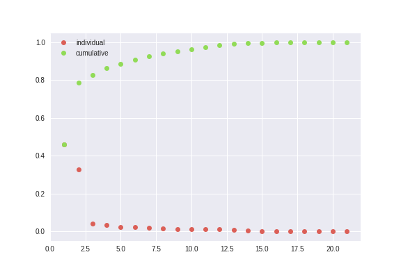
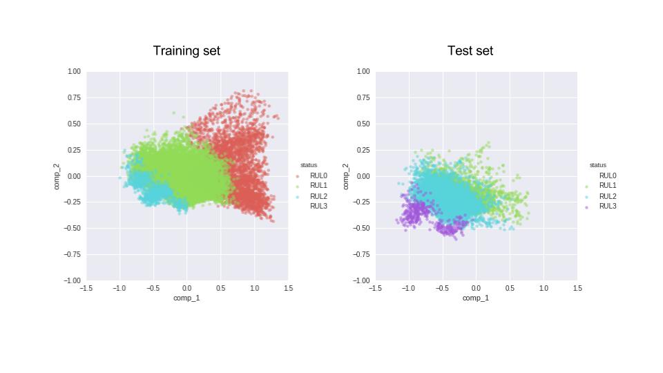
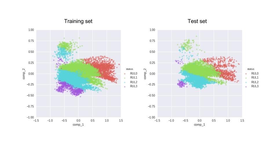
After examining the results of the PCA (and trying a few unsupervised classification on the data, that failed miserably), I decided to merge the provided training and test sets, so that my algorithm gets a chance to learn about all stages of an engine’s health before it has to predict the classes. This is the separation of our 4 classes based on the labels (RULs) for the training and test set. The training set has no instances of RUL but lots of RUL0, while the test set is the opposite (RUL0 corresponds to the last healthy phase of the engine where the RUL is very small, and RUL3 corresponds to the leftmost part of the sequences in figure 1).

Now let’s merge the datasets (and then split them randomly into training, test, and validation sets). So, when it comes to predicting the health stage of the engine, the training algorithm is actually aware of all the n (in this case 4) classes that we have defined.

Next I save the preprocessed data and form now on work with the principal components as my features only.

Preprocessing notebook

Supervised classification

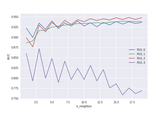
Now that the problem looks more manageable, let’s start with the simples (but not the most practical in real life!) algorithm; the k-nearest neighbor classification. The search on the number of neighbors shows that while the area under the ROC curve starts high and plateau for 3 of the 4 classes with increasing n, the instances of the forth class (RUL3) remain difficult to predict and the best performance happens using abour 3 neighbors for prediction.

Below is scikitlearn’s classification_report for the out-of-the-box KNN algorithm. There is clearly room for improvement, especially for classes 0 and 3. Besides, KNN is not a learning algorithm, i.e. all the computation is done in the inference step, rather than the one-time training phase, which makes it pretty unattractive for most real-life usages.

             precision    recall  f1-score   support

          0       0.85      0.89      0.87       720
          1       0.91      0.93      0.92      3693
          2       0.93      0.90      0.91      2530
          3       0.93      0.74      0.83       145

avg / total       0.91      0.91      0.91      7088

Now let’s see if fully-connected layer can do any better. Here are the results of a fully-connected feed-forward network with 10-units in the first and the only hidden layer, and 20% dropout at each layer.

             precision    recall  f1-score   support

          0       0.91      0.71      0.79       720
          1       0.93      0.98      0.96      3693
          2       0.96      0.97      0.97      2530
          3       1.00      0.44      0.61       145

avg / total       0.94      0.94      0.94      7088

This is already much better than the KNN, and perhaps you can make it better by fine-tuning the parameter in the notebook I am linking in the end of this section too. But why not experiment with different architectures? Below, I am asking an hour-glass network to do the same classification for me. My hourglass has a 10-unit layer as the input layer, then narrows down to two 5 -unit layers, and then back to a 10-unit one before the output layer that has 4 nodes and uses a softmax activation function (sigmoid in case n_classes=2).

             precision    recall  f1-score   support

          0       0.91      0.99      0.95       720
          1       1.00      0.96      0.98      3693
          2       0.92      1.00      0.96      2530
          3       0.00      0.00      0.00       145

avg / total       0.94      0.96      0.95      7088

The hourglass network seems to be ignoring the fourth class, but is doing a considerably better job in the other 3 classes. I am using an early stopping callback in my code, but looking at the learning curve of the hourglass, I suspect that increasing the patience of the early stopper, i.e. letting the hourglass run for more epochs, might help.

Below is the notebook that reproduces these results. There are a few parameters to be set in the second cell. Although not everything is made to be user friendly and you can check out the tools I used to replace the functions that make each of these models using keras and change the parameters of the network there too.

Supervised classification notebook

And last, but not least (actually the most exciting for me as I’m just learning about it!), let’s use a network of Long-Short Term Memory cells to do the same classification job. After spending way too much time than I like to admit, I finally figured out the reshaping that needs to happen before sending sequences to an LSTM network. Now, here is how the LSTM network performs after just 50 epochs! Amazing, isn’t it?

             precision    recall  f1-score   support

          0       0.97      0.95      0.96       720
          1       0.98      0.99      0.99      3178
          2       0.99      1.00      0.99      1878
          3       1.00      0.99      1.00      7504

avg / total       0.99      0.99      0.99     13280

LSTM classification notebook

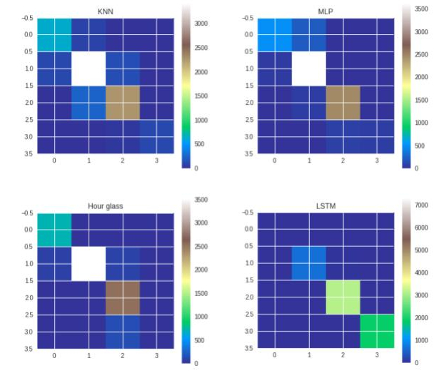
Now let’s have a look at the confusion matrices of all the four methods to have an overview of their performance.

What’s next?

I am trying to get my hands on some real aircraft engine data to do analysis on. From the glimpse I got to have, the format the real data come in is already hard to figure out. Besides, I have not yet figured out how to use the data in manually-collected logs to account for maintenance and possible replacements done in certain parts of the engine and use data that do not include failure events! But as for this data set, I would like to get back to it and try out the seq2seq LSTM on it, now that I already feel comfortable with this dataset. But who knows when a newer, cooler, shinier dataset comes my way and distracts me?